Data Science mit OpenStreetMap
Nikolai Janakiev @njanakiev

Überblick
- Datenakquise
- Datentransformation
- Datenanalyse
- Datenvisualisierung
Datenakquise
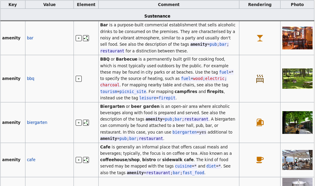
Einrichtungen (Amenities) in OpenStreetMap
- Attribute sind als key-value pairs gespeichert
- Amenity key
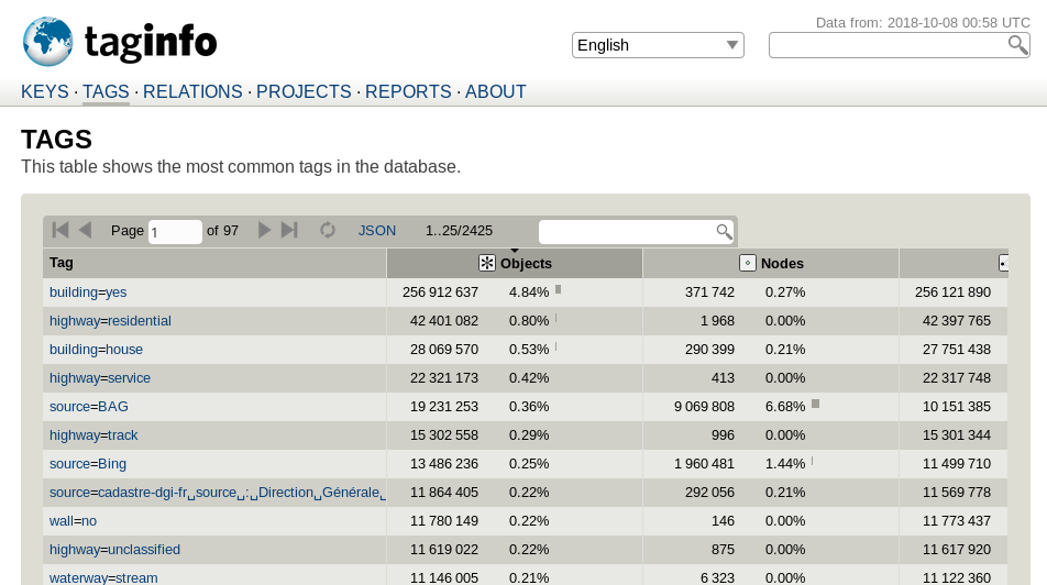
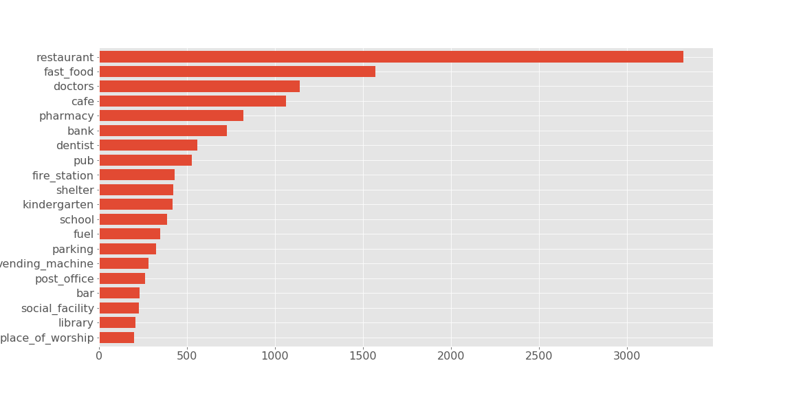
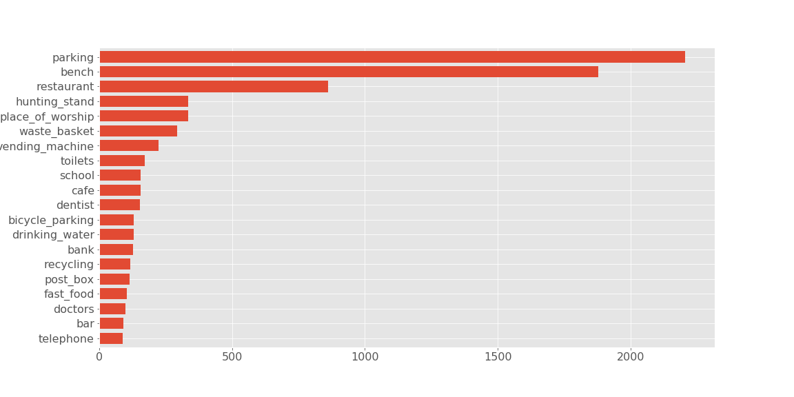
Taginfo Statistiken
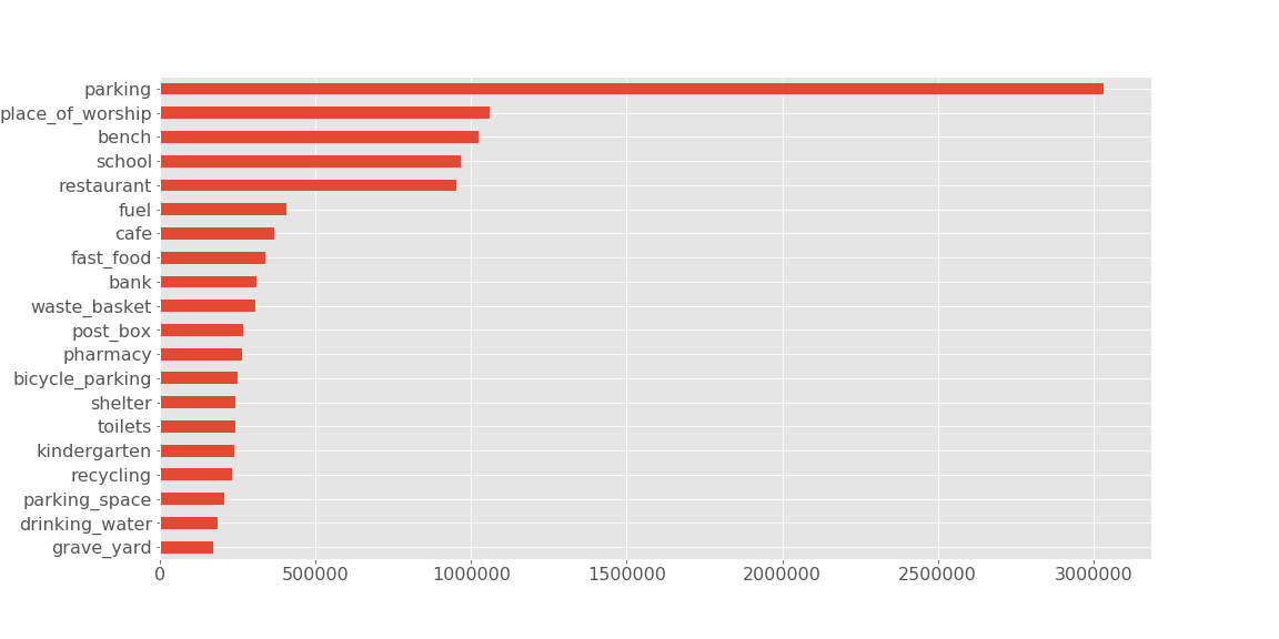
Häufigsten Einrichtungen in OpenStreetMap
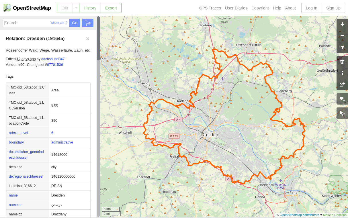
OpenStreetMap Stadt Regionen
Eurostat (Statistische Amt der Europäischen Union)
Overpass API
In [1]:
import requests

overpass_url = "http://overpass-api.de/api/interpreter"
overpass_query = """
    [out:json];
    area["ISO3166-1"="DE"][admin_level=2]->.search;
    node[amenity="restaurant"](area.search);
    out count;"""
response = requests.get(overpass_url, params={'data': overpass_query})
response.json()
Out[1]:
Daten aus OpenStreetMap Dateien Extrahieren
- Dateien aus Geofabrik oder direkt Regionen aus OpenStreetMap exportieren
- Osmium Tool für die Kommandozeile oder PyOsmium mit Python
In [4]:
import osmium

class RestaurantHandler(osmium.SimpleHandler):
    def __init__(self):
        osmium.SimpleHandler.__init__(self)
        self.num_restaurants = 0

    def node(self, n):
        if n.tags.get('amenity') == 'restaurant':
            self.num_restaurants += 1

handler = RestaurantHandler()
handler.apply_file('data/liechtenstein-latest.osm.pbf')
print('Number of Restaurants: ', handler.num_restaurants)
Datentransformation
Installation
conda install -c conda-forge geopandas
Laden von Geodaten von PostGIS
In [6]:
import psycopg2
import geopandas as gpd

with psycopg2.connect(database="osm_data_science", user="postgres",
                      password='password', host='localhost') as connection:

    gdf = gpd.GeoDataFrame.from_postgis(
        """SELECT osm_id, amenity, state, geom FROM osm_amenities_areas""",
        connection, geom_col='geom')

gdf.head()
Out[6]:
Alle Einrichtungen in Österreich
In [7]:
gdf.to_crs({'init': 'epsg:31287'}).plot(
    figsize=(20, 10), alpha=0.4, markersize=0.5, color='k');

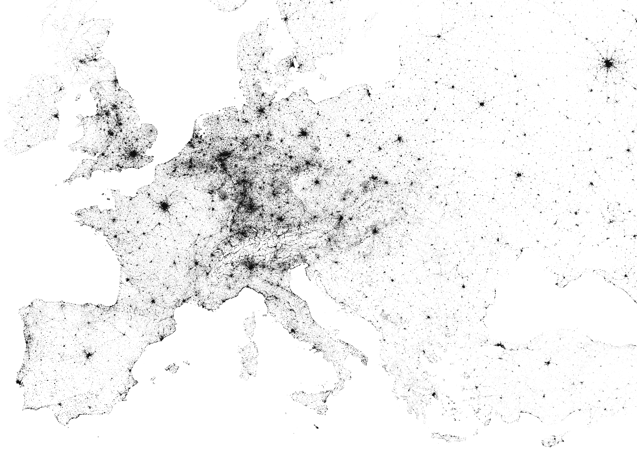
Alle Einrichtungen in Europa
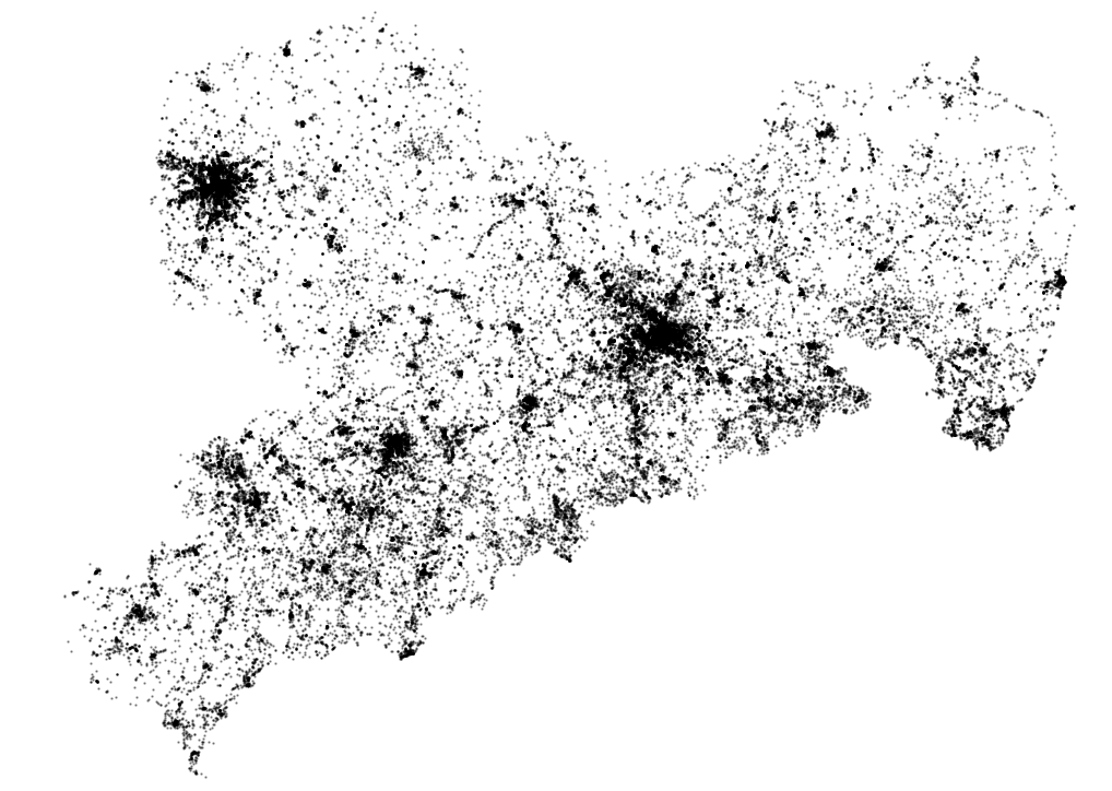
Alle Einrichtungen in Sachsen
Datenanalyse
Was sind die Häufigsten Einrichtungen in Sachsen?
Was sind die Häufigsten Einrichtungen in Salzburg Land?
Was macht eine Französische/Deutsche Stadt oder Region aus?
Statistische Klassifizierung
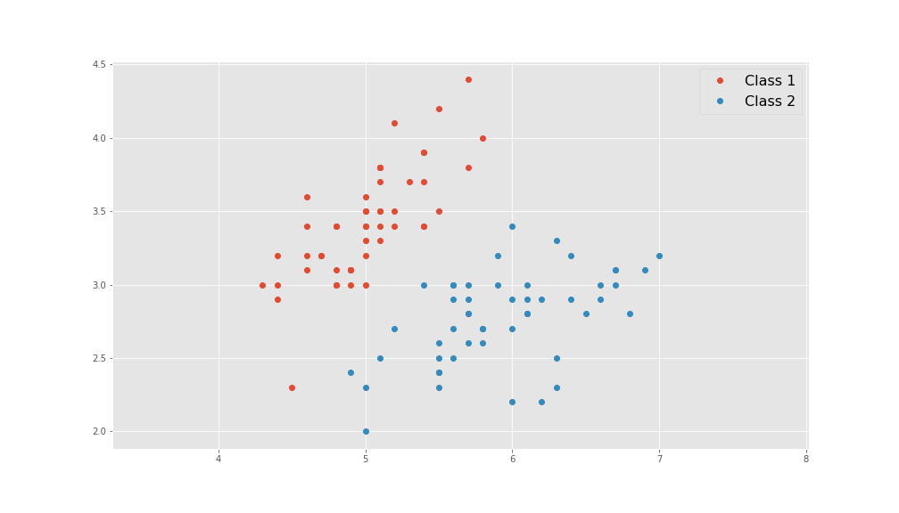
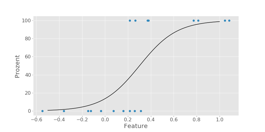
Logistische Regression
Laden und Vorbereitung der Daten
In [1]:
import psycopg2
import geopandas as gpd

with psycopg2.connect(database="osm_data_science", user="postgres",
                      password='postgres', host='localhost') as connection:
    gdf = gpd.GeoDataFrame.from_postgis(
            "SELECT * FROM city_amenity_counts",
            connection, geom_col='geom')

gdf.loc[:, 'parking':'veterinary'].head()
Out[1]:
In [2]:
# Get only Germany and France
gdf_DE_FR = gdf[(gdf['country_code'] == 'DE') | \
                (gdf['country_code'] == 'FR')].copy()
Die Feature Vektoren und Klassen wählen
In [3]:
X = gdf_DE_FR.loc[:, 'parking':'veterinary'].values
y = gdf_DE_FR['country_code'].map({'DE': 0, 'FR': 1}).values
In Training und Test Datensatz aufteilen
In [4]:
from sklearn.model_selection import train_test_split

X_train, X_test, y_train, y_test = train_test_split(
    X, y, test_size=0.3, random_state=1000)
Logistische Regression mit Scikit-Learn
In [9]:
from sklearn.linear_model import LogisticRegressionCV

clf = LogisticRegressionCV(cv=5)
clf.fit(X_train, y_train)
Out[9]:
In [10]:
print('Training score : {:.4f}'.format(clf.score(X_train, y_train)))
print('Testing score  : {:.4f}'.format(clf.score(X_test, y_test)))
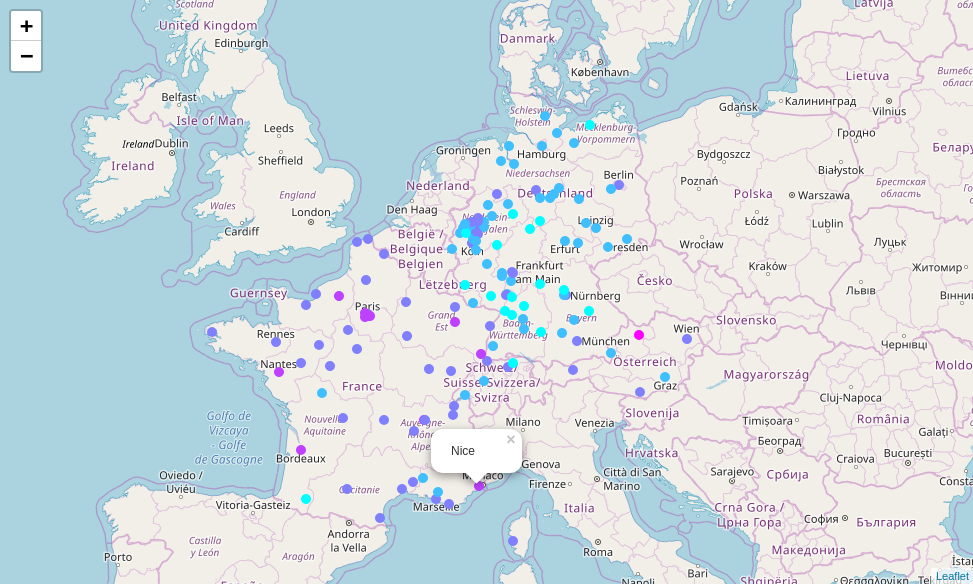
Berechne die Wahrscheinlichkeit dass eine Stadt Französisch ist
In [11]:
gdf['frenchness'] = gdf.loc[:, 'parking':'veterinary'].apply(
    lambda row: clf.predict_proba([row.values])[:, 1][0], axis=1)
Datenvisualisierung
Visualisierung mit Folium
- Visualisierungsbibliothek mit Leaflet.js
In [22]:
import folium
import matplotlib

cmap = matplotlib.cm.get_cmap('cool', 5)

m = folium.Map(location=[49.5734053, 7.588576], zoom_start=5)
for i, row in gdf.iterrows():

    rgb = cmap(row['frenchness'])[:3]
    hex_color = matplotlib.colors.rgb2hex(rgb)

    folium.CircleMarker([row['geom'].y, row['geom'].x],
                        radius=5, popup=row['city'],
                        fill_color=hex_color, fill_opacity=1,
                        opacity=0.0).add_to(m)
m.save('maps/folium_map.html')
In [3]:
from IPython.display import IFrame

IFrame('maps/folium_map.html', width=1024, height=600)
Out[3]:
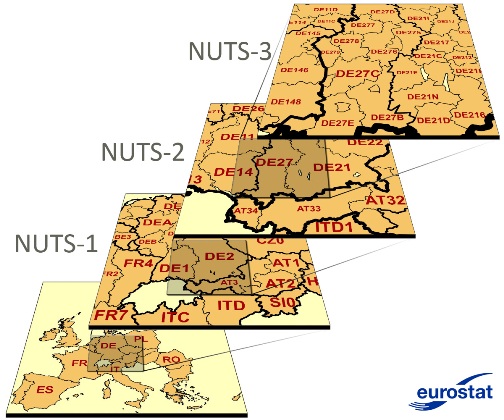
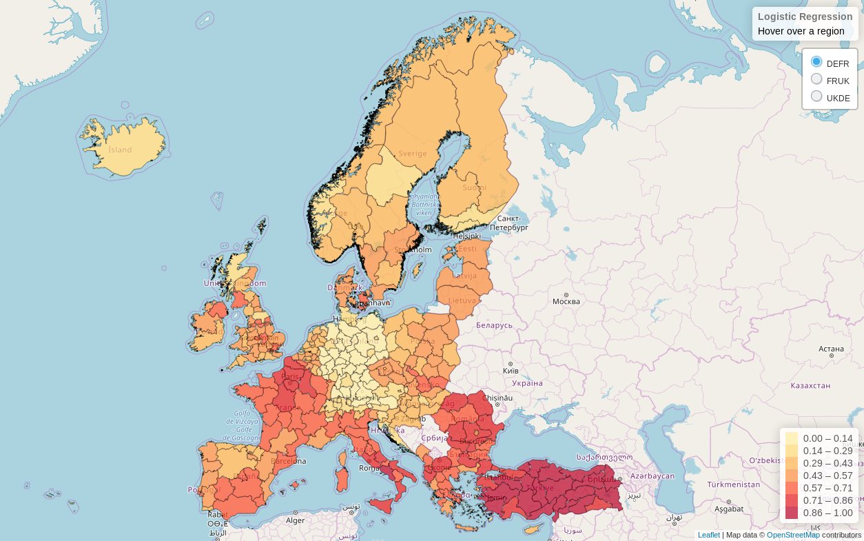
Logistische Regression anhand von Eurostat NUTS Regionen
Data Science mit OpenStreetMap
Nikolai Janakiev @njanakiev
- Visualization @ osm.janakiev.com/
- Slides @ janakiev.com/osm-data-science/
- Repository @ github.com/njanakiev/osm-data-science